MACD Volume VWAP Scalping (2min) by Obiii📘 Strategy Description (for TradingView)
MACD Volume VWAP Scalping Strategy (2-Minute Intraday Momentum)
This strategy is designed for scalpers and short-term intraday traders who focus on capturing small, high-probability moves during the most active hours of the trading session — typically between 9:45 AM and 11:30 AM (New York time).
The system combines three key momentum confirmations:
MACD crossovers to detect short-term trend shifts,
Volume spikes to validate real market participation, and
VWAP / EMA alignment to filter trades in the direction of the prevailing intraday trend.
🔹 Entry Logic
Long Entry:
MACD line crosses above the signal line
Both MACD and Signal are above zero
Current volume > average of the last 10 candles
Price is above VWAP and (optionally) above EMA 9 and EMA 20
Short Entry:
MACD line crosses below the signal line
Both MACD and Signal are below zero
Current volume > average of the last 10 candles
Price is below VWAP and (optionally) below EMA 9 and EMA 20
🎯 Exit Logic
Fixed Take Profit: +0.25%
Fixed Stop Loss: -0.15% to -0.20%
Optionally, switch to the 5-minute chart after entry to monitor momentum and manage exits more smoothly.
⚙️ Recommended Settings
Timeframe: 2 minutes (entries), 5 minutes (monitoring)
Market Session: 9:45 AM – 11:30 AM EST
Assets: Highly liquid instruments such as SPY, QQQ, NVDA, TSLA, AAPL, or large-cap momentum stocks.
💡 Notes
This is a momentum-based scalping strategy — precision and discipline are key.
It performs best in high-volume environments where clear direction emerges after the morning volatility settles.
The system can be fine-tuned for different profit targets, MACD settings, or volume thresholds depending on volatility.
Поиск скриптов по запросу "take profit"

Pearson SL/TP📘 Description
Pearson SL/TP — Advanced Correlation-Based Strategy with Full Risk Management
The Pearson SL/TP indicator is an advanced market analysis tool that combines Pearson correlation, volatility-based stop/target levels, and dynamic signal strength evaluation.
It is designed for traders who want to visualize potential momentum shifts and risk/reward zones in a single, integrated chart.
🔍 Core Concept
This script measures the **Pearson correlation coefficient between recent price movements and time progression, highlighting potential trend exhaustion or momentum reversals when the correlation reaches extreme values.
* High positive correlation (near +1) → price moving steadily upward → possible overbought condition.
* High negative correlation (near -1) → price moving steadily downward → possible oversold condition.
When these extremes are reached, and confirmed by several internal filters, the script generates LONG or SHORT signals with fully calculated Stop Loss and Take Profit levels.
⚙️ Main Features
📈 Signal Generation
* Uses Pearson correlation as a primary indicator of trend intensity.
* Detects potential reversal zones when correlation crosses user-defined thresholds.
* Optional divergence confirmation enhances signal reliability.
💰 Risk Management
* Stop Loss (SL) and Take Profits (TP1 & TP2) automatically adapt to volatility using the ATR (Average True Range).
* Dynamic risk/reward ratios help assess trade quality.
* Adjustable multipliers let you fine-tune your risk parameters.
🧠 Signal Strength Analysis
Each signal is graded from Weak to Very Strong based on four factors:
1. Volume activity
2. Trend alignment
3. Pearson momentum
4. Correlation change intensity
🎨 Visualization
* Overbought / Oversold background zones
* Signal arrows (LONG / SHORT)
* SL / TP** price levels and labels
* Interactive dashboard** displaying:
* Current Pearson value
* Market state (Overbought / Oversold / Neutral)
* Signal strength
* Latest trade data (Entry, SL, TP1, TP2, Risk:Reward)
🔔 Alerts
Built-in alerts for:
* Confirmed LONG / SHORT signals
* Bullish / Bearish divergences
🧩 Customization
All major parameters — including **Pearson length, thresholds, ATR multipliers, and visual options — are fully customizable.
This allows you to adapt the indicator to any market, timeframe, or trading style.

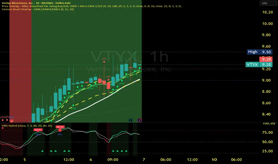
Victoria RSI Hybrid Pro – Momentum + Volume + DivergenceConditions and Actions:
RSI > 50 → Bullish regime → Consider Calls
RSI < 50 → Bearish regime → Consider Puts
RSI crosses up → Momentum shift up → Buy confirmation
RSI crosses down → Momentum shift down → Sell confirmation
RSI > 70 → Overbought → Take profits
RSI < 30 → Oversold → Watch for reversal
Bullish divergence → Hidden upward momentum → Reversal watch
Bearish divergence → Hidden downward momentum → Reversal watch
4. Multi-Indicator Confirmation Rules
Combine signals from EMA, SMA, RSI, and Volume to identify high-confidence trades.
Rules:
Triple Green → EMA1>SMA3, RSI>50, Volume Up → Buy Calls / Shares
Triple Red → EMA1 70 + Weak Volume → Exit Calls early
EMA1 flips direction + Strong Volume → Confirm bias immediately
RSI on 1H agrees with main chart → Trend continuation likely
6. Timeframes
Scalps: 1m–5m
Next-Day Options: 15m–1H
Swings: 4H–1D
7. Key Mindset Rules
Patience beats prediction. Wait for confirmations.
Volume confirms conviction, not direction.
If RSI and Overlay disagree → No trade.
Only act when 2 of 3 systems (EMA, RSI, Volume) align.
Tristan's Multi-Indicator Reversal StrategyMulti-Indicator Reversal Strategy - Buy Low, Sell High
A comprehensive reversal detection system that combines multiple proven technical indicators to identify high-probability entry points for catching reversals at market extremes.
📊 Strategy Overview
This strategy is designed for traders who want to buy at lows and sell at highs by detecting when stocks are overextended and ready to reverse. It works by requiring multiple technical indicators to align before generating a signal, significantly reducing false entries.
Best Used On:
Timeframe: 1-hour charts (also works on 15min, 30min, 4hour)
Session: NY Trading Session (9:30 AM - 4:00 PM ET)
Assets: Stocks, ETFs, Crypto (particularly volatile tech stocks like ZM, TSLA, AAPL)
Trading Style: Swing trading, Intraday reversals
🔧 Technical Components
The strategy combines FIVE powerful technical indicators:
1. RSI (Relative Strength Index)
2. MACD (Moving Average Convergence Divergence)
3. Williams %R
4. Bollinger Bands
5. Volume Analysis
6. Divergence Detection (Optional)
🎨 Visual Signals
Entry Signals:
🟢 Green Triangle (below candle) = BUY LONG signal
🔴 Red Triangle (above candle) = SELL SHORT signal
Exit Signals:
🟣 Purple Label = Position closed (shows "x2", "x3" if multiple entries)
Additional Indicators:
💎 Aqua Diamond = Bullish divergence detected
💎 Fuchsia Diamond = Bearish divergence detected
🔵 Blue Background = NY Session active
🟡 Yellow Bar Tint = Volume spike detected
⚪ Small Circles = Near-signal conditions (2+ indicators aligned)
Live Counter:
Top corner shows: "Bull: X/4" and "Bear: X/4"
Indicates how many indicators currently align
⚙️ How to Use This Strategy
For Beginners (More Signals):
Set "Min Indicators Aligned" to 2
Turn OFF "Require Divergence"
Turn OFF "Require Volume Spike"
Turn OFF "Require Reversal Candle Pattern"
Keep "Allow Multiple Entries" OFF
This gives you more frequent signals to learn from.
For Advanced Traders (High Probability):
Set "Min Indicators Aligned" to 3 or 4
Turn ON "Require Divergence"
Turn ON "Require Volume Spike"
Turn ON "Require Reversal Candle Pattern"
Adjust stop loss to your risk tolerance
This filters for only the highest-quality setups.
Recommended Settings for 1-Hour Charts:
Min Indicators Aligned: 3
Stop Loss: 2.5%
Take Profit: 5.0%
RSI Length: 14
Williams %R Length: 14
Volume Multiplier: 1.5x
Session: NY only (for stocks)
BUY SIGNAL generated when:
2-4 indicators show oversold/bullish conditions:
RSI < 30 and turning up
MACD crossing bullish or histogram positive
Williams %R < -80 and turning up
Price at/below lower Bollinger Band
Optional confirmations (if enabled):
Bullish divergence detected
Volume spike present
Bullish reversal candle pattern
Session filter: Signals only during NY trading hours
SELL SIGNAL Generated When:
2-4 indicators show overbought/bearish conditions:
RSI > 70 and turning down
MACD crossing bearish or histogram negative
Williams %R > -20 and turning down
Price at/above upper Bollinger Band
Optional confirmations (if enabled):
Bearish divergence detected
Volume spike present
Bearish reversal candle pattern
🛡️ Risk Management Features
Automatic Stop Loss: Protects capital (default 2.5%)
Take Profit Target: Locks in gains (default 5.0%)
Pyramiding Control: Toggle to prevent position stacking
Session Filter: Avoids overnight risk and low-liquidity periods
Position Flipping: Automatically reverses when opposite signal appears
💡 Best Practices
✅ DO:
Wait for candle close before entering (built into strategy)
Use on volatile assets with clear trends
Combine with your own analysis and risk management
Backtest on your specific assets and timeframes
Start with paper trading to learn the signals
Adjust indicator requirements based on market conditions
❌ DON'T:
Use on very low timeframes (<5 min) without adjustment
Ignore the session filter on stocks
Use maximum leverage - these are reversal trades
Trade during major news events or earnings
Expect 100% win rate - focus on risk/reward ratio
📊 Performance Notes
This strategy prioritizes quality over quantity. With default settings, you may see:
2-5 signals per week on 1-hour charts
Higher win rate with stricter settings (3-4 indicators aligned)
Best performance during trending markets with clear reversals
Reduced performance in choppy, sideways markets
Tip: Adjust "Min Indicators Aligned" based on market conditions:
Trending markets: Use 3-4 (fewer but stronger signals)
Range-bound markets: Use 2 (more signals, but watch for false breakouts)

Trend Pullback System```{"variant":"standard","id":"36492","title":"Trend Pullback System Description"}
Trend Pullback System is a price-action trend continuation model that looks to enter on pullbacks, not breakouts. It’s designed to find high-quality long/short entries inside an already established trend, place the stop at meaningful structure, trail that stop as structure evolves, and warn you when the trade thesis is no longer valid.
Developed by: Mohammed Bedaiwi
---------------------------------
HOW IT WORKS
---------------------------------
1. Trend Detection
• The strategy defines overall bias using moving averages.
• Bullish environment (“uptrend”): price above the slower MA, fast MA above slow MA, and the slow MA is sloping up.
• Bearish environment (“downtrend”): price below the slower MA, fast MA below slow MA, and the slow MA is sloping down.
This prevents trading against chop and focuses on continuation moves in the dominant direction.
2. Pullback + Re-entry Logic
• The script waits for price to pull back into structure (support in an uptrend, resistance in a downtrend), and then push back in the direction of the main trend.
• That “push back” is the setup trigger. We don’t chase the first breakout candle — we buy/sell the retest + resume.
3. Structural Levels (“Diamonds”)
• Green diamond (below bar): bullish pivot low formed while the trend is bullish. This marks defended support.
- Use it as a re-entry zone for longs.
- Use it to trail a stop higher when you’re already long.
- Shorts can take profit here because buyers stepped in.
• Red diamond (above bar): bearish pivot high formed while the trend is bearish. This marks defended resistance.
- Use it as a re-entry zone for shorts.
- Use it to trail a stop lower when you’re already short.
- Longs can take profit here because sellers stepped in.
4. Entry Signals
• BUY arrow (green triangle up under the candle, text like “BUY” / “BUY Zone”):
- LongSetup is true.
- Trend is bullish or turning bullish.
- Price just bounced off recent defended support (green diamond) and reclaimed short-term momentum.
Meaning: enter long here or cover/exit shorts.
• SELL arrow (red triangle down above the candle):
- ShortSetup is true.
- Trend is bearish or turning bearish.
- Price just rolled down from defended resistance (red diamond) and lost short-term momentum.
Meaning: enter short here or take profit on longs.
These are the primary trade entries. They are meant to be actionable.
5. Weak Setups (“W” in yellow)
• Yellow triangle with “W”:
- A possible long/short idea is trying to form, BUT the higher-timeframe confirmation is not fully there yet.
- Think of it as early pressure / early caution, not a full signal.
• You usually watch these areas rather than jumping in immediately.
6. Exit Warning (orange “EXIT” label above a bar)
• The strategy will raise an EXIT marker when you’re in a trade and the *opposite* side just produced a confirmed setup.
- You’re short and a valid longSetup appears → EXIT.
- You’re long and a valid shortSetup appears → EXIT.
• This is basically: “Close or reduce — the other side just took control.”
• It’s not just a trailing stop hit; it’s a regime flip warning.
7. Stop, Target, and Trailing
• On every new setup, the script records:
- Initial stop: recent swing beyond the defended level (below support for longs, above resistance for shorts).
- Initial target: recent opposing swing.
• While you’re in position, if new confirming diamonds print in your favor, the stop can trail toward the new defended level.
• This creates structure-based risk management (not just fixed % or ATR).
8. Reference Levels
• The strategy also plots prior higher-timeframe closes (last week’s close, last month’s close, last year’s close). These can behave as magnets or stall points.
• They’re helpful for take-profit timing and for reading “are we trading above or below last month’s close?”
9. Momentum Panel (hidden by default)
• Internally, the script calculates an SMI-style momentum oscillator with overbought/oversold zones.
• This is optional visual confirmation and does not drive the core entry/exit logic.
---------------------------------
WHAT A TRADE LOOKS LIKE IN REAL PRICE ACTION
---------------------------------
Early warning
• Yellow W + red diamonds + red down arrows = “This is getting weak. Short setups are here.”
• You may also see something like “My Short Entry Id.” That’s where the short side actually engages.
Bearish follow-through, then exhaustion
• Price bleeds down.
• Then the orange EXIT appears.
→ Translation: “If you’re still short, close it. Buyers are stepping in hard. Risk of reversal is now high.”
Regime flip
• Right after EXIT, multiple green BUY arrows fire together (“BUY”, “BUYZone”).
• That’s the true long trigger.
→ This is where you either enter long or flip from short to long.
Expansion leg
• After that flip, price rips up for multiple candles / days / weeks.
• While it runs:
- Green diamonds appear under pullbacks → “dip buy zones / trail stop up here.”
- More BUY arrows show on minor pullbacks → continuation long / scale adds.
Distribution / topping
• Later, you start seeing new yellow W triangles again near local highs. That’s your “careful, this might be topping” warning.
• You finally get a hard red candle, and green diamonds stop stacking.
→ That’s where you tighten risk, scale out, or assume the move is mature.
In plain terms, the model is doing the following for you:
• It puts you short during weakness.
• It tells you when to get OUT of the short.
• It flips you long right as control changes.
• It gives you a structure-based trail the whole way up.
• It warns you again when momentum at the top starts cracking.
That is exactly how the logic was designed.
---------------------------------
QUICK INTERPRETATION CHEAT SHEET
---------------------------------
🔻 Red triangle + “Short Entry” near a red diamond
→ Short entry zone (or take profit on a long).
🟥 Red diamond above bar
→ Sellers defended here. Treat it as resistance. Good place to trail short stops just above that level. Avoid chasing longs straight into it.
🟨 Yellow W
→ Attention only. Early pressure / possible turn. Not fully confirmed.
🟧 EXIT (orange label)
→ The opposite side just printed a real setup. Close the old idea (cover shorts if you’re short, exit longs if you’re long). Thesis invalid.
🟩 Burst of green BUY triangles after EXIT
→ Long entry. Also a “cover shorts now” alert. This is the core money entry in bullish reversals.
💎 Green diamond below bar
→ Bulls defended that level. Good for trailing your long stop up, and good “buy the dip in trend” locations.
📈 Blue / teal MAs stacked and rising
→ Confirmed bullish structure. You’re in trend continuation mode, so dips are opportunities, not automatic exits.
---------------------------------
COLOR / SHAPE KEY
---------------------------------
• Green triangle up (“BUY”, “BUY Zone”):
Long entry / cover shorts / continuation long trigger.
• Red triangle down:
Short entry / take profit on longs / continuation short trigger.
• Orange “EXIT” label:
Opposite side just fired a real setup. The previous trade thesis is now invalid.
• Green diamond below price:
Bullish defended support in an uptrend. Use for dip buys, trailing stops on longs, and objective cover zones for shorts.
• Red diamond above price:
Bearish defended resistance in a downtrend. Use for re-entry shorts, trailing stops on shorts, and objective scale-out zones for longs.
• Yellow “W”:
Weak / early potential setup. Watch it, don’t blindly trust it.
• Moving average bands (fast MA, slow MA, Hull MA):
When stacked and rising, bullish control. When stacked and falling, bearish control.
---------------------------------
INTENT
---------------------------------
This system is built to:
• Trade with momentum, not against it.
• Enter on pullbacks into proven structure, not chase stretched breakouts.
• Automate stop/target logic around actual defended swing levels.
• Warn you when the other side takes over so you don’t give back gains.
Typical usage:
1. In an uptrend, wait for price to pull back, print a green diamond (support proved), then take the first BUY arrow that fires.
2. In a downtrend, wait for a bounce into resistance, print a red diamond (sellers proved), then take the first SELL arrow that fires.
3. Respect EXIT when it appears — that’s the model saying “this trade is done.”
---------------------------------
DISCLAIMER
---------------------------------
This script is for educational and research purposes only. It is not financial advice, investment advice, or a recommendation to buy or sell any security, cryptoasset, or derivative. Markets carry risk. Past performance does not guarantee future results. You are fully responsible for your own decisions, position sizing, risk management, and compliance with all applicable laws and regulations.

[Kpt-Ahab] Assistant: Risk & DCA PlannerScript Description – Assistant: Risk & DCA Planner
The Risk & DCA Planner is a technical assistant for position and risk management.
It automatically calculates, based on volatility (ATR%), swing structure, and your settings:
Stop-Loss (SL) and corresponding Take-Profit targets (TPs) in R-multiples
DCA (Dollar-Cost-Averaging) levels — both price and amount
A market suitability check (based on volatility & volume)
Plus a clear table and summary label displayed on the chart
The script helps you plan risk, scaling, and profit targets consistently and quantitatively.
Core Logic
Risk Profile
Three modes: Low, Normal, High.
These define how reactive the script behaves internally:
Low → conservative, longer lookbacks, tighter analysis
Normal → balanced
High → aggressive, faster reaction, wider stops
Stop-Loss (SL)
Automatically calculated from ATR% and recent swing structure, limited by minimum and maximum thresholds.
The SL percentage defines the R-unit, which all TPs and DCA levels are based on.
Take-Profits (TPs)
Up to six targets, each a multiple of the defined risk (e.g., 1R, 2R, 3R).
Prices are automatically adjusted depending on long or short direction.
DCA Strategy
Optional. Adds scaling levels evenly between Entry and SL or in multiples of the ATR.
Each DCA allocation grows geometrically until the maximum position size is reached.
Suitability Check
Evaluates whether the market is within an appropriate ATR% range and has sufficient volume.
The table displays “OK” or “Caution” depending on volatility and historical consistency.
Visualization
Lines for SL, TPs, and DCA levels
A table with all parameters, prices, and risk data
A chart label summarizing key info (profile, direction, SL%, TPs, DCA, etc.)

Advanced Multi-Timeframe Trend & Signal System═══════════════════════════════════════════════════════════════
ADVANCED MULTI-TIMEFRAME TREND & SIGNAL SYSTEM v1.0
═══════════════════════════════════════════════════════════════
Created by: Zakaria Safri
License: Mozilla Public License 2.0
A comprehensive technical analysis tool designed for traders seeking
multi-dimensional market insights. This indicator combines proven
technical analysis methods with modern visualization techniques.
═══════════════════════════════════════════════════════════════
KEY FEATURES
═══════════════════════════════════════════════════════════════
✓ SUPERTREND SIGNAL GENERATION
- Customizable sensitivity settings
- Clear long/short entry signals
- Automatic trend direction detection
- ATR-based dynamic calculations
✓ MULTI-TIMEFRAME DASHBOARD
- Real-time trend analysis across 6 timeframes
- Synchronized trend confirmation
- Customizable table position and size
- Current: 1M, 5M, 15M, 1H, 1D coverage
✓ QQE REVERSAL DETECTION
- Quantitative Qualitative Estimation algorithm
- Early reversal signal identification
- Adjustable RSI and smoothing parameters
- Confirmation-based plotting
✓ DYNAMIC SUPPORT & RESISTANCE
- Pivot-based level calculation
- Quick and standard pivot detection
- Color-coded zones (8 levels)
- Automatic level updates
✓ MOMENTUM BREAKOUT SIGNALS
- Ichimoku-inspired calculations
- Bullish and bearish breakout detection
- Visual zone highlighting
- Trend confirmation filters
✓ RISK MANAGEMENT SYSTEM
- ATR-based stop loss calculation
- Multiple take profit targets (TP1, TP2, TP3)
- Customizable risk-to-reward ratios
- Dynamic price level tracking
- Hit detection markers
✓ VOLATILITY BANDS
- Keltner Channel implementation
- Multiple band layers (3 levels)
- EMA-based calculations
- Adaptive to market conditions
✓ TREND CLOUD VISUALIZATION
- Dual moving average cloud
- Clear trend direction indication
- Customizable color scheme
- Trend bar coloring
═══════════════════════════════════════════════════════════════
HOW TO USE
═══════════════════════════════════════════════════════════════
SETUP:
1. Add indicator to your chart
2. Configure sensitivity in Core Signals section
3. Enable desired features (signals, reversals, breakouts)
4. Set up risk management levels if trading
5. Position MTF dashboard to preference
SIGNAL INTERPRETATION:
• LONG Signal: Price crosses above Supertrend
• SHORT Signal: Price crosses below Supertrend
• REV (Reversal): QQE indicates potential trend change
• Diamond Breakouts: Momentum shift confirmation
• T1/T2/T3: Take profit level hits
MULTI-TIMEFRAME ANALYSIS:
• Green (BULL): Higher timeframe supports uptrend
• Red (BEAR): Higher timeframe supports downtrend
• Use for trend alignment and confirmation
• Best results when multiple timeframes align
RISK MANAGEMENT:
• Enable Stop Loss for automatic SL calculation
• Activate TP levels based on trading style
• Adjust Risk-to-Reward ratio (1:1 to 1:10)
• Monitor hit detection circles for exits
═══════════════════════════════════════════════════════════════
TECHNICAL SPECIFICATIONS
═══════════════════════════════════════════════════════════════
CALCULATIONS:
• Supertrend: ATR-based with customizable multiplier
• QQE: Modified RSI with Wilders smoothing
• Keltner Channels: EMA basis with ATR bands
• Pivots: Standard left/right bar methodology
• Support/Resistance: Multi-level pivot analysis
PARAMETERS:
• Supertrend Sensitivity: 0.5 to 10.0 (default: 2.0)
• RSI Period: 5 to 50 (default: 14)
• QQE Multiplier: 1.0 to 10.0 (default: 4.238)
• Risk-to-Reward: 1 to 10 (default: 4)
TIMEFRAMES:
Compatible with all timeframes. MTF dashboard displays:
• 1 Minute (1M)
• 5 Minutes (5M)
• 15 Minutes (15M)
• 1 Hour (1H)
• 1 Day (1D)
• Current chart timeframe
═══════════════════════════════════════════════════════════════
CUSTOMIZATION OPTIONS
═══════════════════════════════════════════════════════════════
VISUAL:
• Professional color scheme (Cyan/Orange)
• Adjustable table position (9 positions)
• Table size options (tiny/small/normal/large)
• Transparent zone highlighting
• Clean, modern label design
TOGGLES:
• Enable/disable any feature independently
• Show/hide signals, reversals, breakouts
• Toggle S/R levels and zones
• Control trend cloud and bands
• Master trend line optional
ALERTS:
The indicator provides visual signals that can be used with
TradingView's alert system by setting alerts on the indicator.
═══════════════════════════════════════════════════════════════
BEST PRACTICES
═══════════════════════════════════════════════════════════════
✓ Combine signals for higher probability setups
✓ Use MTF dashboard for trend confirmation
✓ Respect S/R levels for entry/exit planning
✓ Monitor QQE reversals at key price levels
✓ Adjust sensitivity based on asset volatility
✓ Test on demo/paper trading first
✓ Use proper risk management always
═══════════════════════════════════════════════════════════════
IMPORTANT DISCLAIMER
═══════════════════════════════════════════════════════════════
This indicator is a technical analysis tool and does NOT:
• Guarantee profitable trades
• Provide financial advice
• Predict future price movements with certainty
• Replace proper risk management
• Substitute for personal due diligence
Past performance does not indicate future results. All trading
involves risk. Users should:
- Understand the indicator's logic
- Test thoroughly before live trading
- Use appropriate position sizing
- Never risk more than they can afford to lose
- Consult financial advisors if needed
═══════════════════════════════════════════════════════════════
CODING STANDARDS
═══════════════════════════════════════════════════════════════
This indicator follows PineCoders Coding Conventions:
✓ Proper variable naming (prefixes: i_, f_, c_)
✓ Clear function documentation
✓ Organized code structure
✓ Type declarations
✓ Efficient calculations
✓ No repainting (confirmed signals)
✓ Proper use of request.security
═══════════════════════════════════════════════════════════════
SUPPORT & UPDATES
═══════════════════════════════════════════════════════════════
Version: 1.0
Author: Zakaria Safri
License: MPL 2.0
Last Updated: 2024
For questions, feedback, or suggestions, please comment below.
═══════════════════════════════════════════════════════════════
#trading #signals #supertrend #multiTimeframe #QQE #reversals
#supportResistance #riskManagement #trendAnalysis #momentum

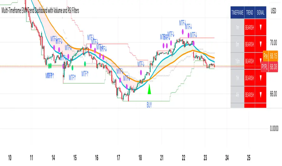
Multi-Timeframe EMA Trend Dashboard with Volume and RSI Filters═══════════════════════════════════════════════════════════
MULTI-TIMEFRAME EMA TREND DASHBOARD
═══════════════════════════════════════════════════════════
OVERVIEW
This indicator provides a comprehensive view of trend direction across multiple timeframes using the classic EMA 20/50 crossover methodology, enhanced with volume confirmation and RSI filtering. It aggregates trend information from six timeframes into a single dashboard for efficient market analysis.
The indicator is designed for educational purposes and to assist traders in identifying potential trend alignments across different time horizons.
═══════════════════════════════════════════════════════════
FEATURES
═══════════════════════════════════════════════════════════
MULTI-TIMEFRAME ANALYSIS
• Monitors 6 timeframes simultaneously: 1m, 5m, 15m, 1H, 4H, 1D
• Each timeframe analyzed independently using request.security()
• Non-repainting implementation with proper lookahead settings
• Calculates overall trend strength as percentage of bullish timeframes
EMA CROSSOVER SYSTEM
• Fast EMA (default: 20) and Slow EMA (default: 50)
• Bullish: Fast EMA > Slow EMA
• Bearish: Fast EMA < Slow EMA
• Neutral: Fast EMA = Slow EMA (rare condition)
• Visual EMA plots with optional fill area
VOLUME CONFIRMATION
• Optional volume filter for crossover signals
• Compares current volume against moving average (default: 20-period SMA)
• Categorizes volume as: High (>1.5x average), Normal (>average), Low (70), oversold (<30), and neutral zones
• Used in quality score calculation
• Optional display toggle
SUPPORT & RESISTANCE DETECTION
• Automatic detection using highest/lowest over lookback period (default: 50 bars)
• Plots resistance (red), support (green), and mid-level (gray)
• Step-line style for clear visualization
• Optional display toggle
QUALITY SCORING SYSTEM
• Rates trade setups from 1-5 stars
• Considers: MTF alignment, volume confirmation, RSI positioning
• 5 stars: 4+ timeframes aligned + volume confirmed + RSI 50-70
• 4 stars: 4+ timeframes aligned + volume confirmed
• 3 stars: 3+ timeframes aligned
• 2 stars: Exactly 3 timeframes aligned
• 1 star: Other conditions
VISUAL DASHBOARD
• Clean table display (position customizable)
• Color-coded trend indicators (green/red/yellow)
• Extended statistics panel (toggleable)
• Shows: Trends, Strength, Quality, RSI, Volume, Price Distance
═══════════════════════════════════════════════════════════
TECHNICAL SPECIFICATIONS
═══════════════════════════════════════════════════════════
CALCULATIONS
Trend Determination per Timeframe:
• request.security() fetches EMA values with gaps=off, lookahead=off
• Compares Fast EMA vs Slow EMA
• Returns: 1 (bullish), -1 (bearish), 0 (neutral)
Trend Strength:
• Counts number of bullish timeframes
• Formula: (bullish_count / 6) × 100
• Range: 0% (all bearish) to 100% (all bullish)
Price Distance from EMA:
• Formula: ((close - EMA) / EMA) × 100
• Positive: Price above EMA
• Negative: Price below EMA
• Warning when absolute distance > 5%
ANTI-REPAINTING MEASURES
• All request.security() calls use lookahead=barmerge.lookahead_off
• Dashboard updates only on barstate.islast
• Historical bars remain unchanged
• Crossover signals finalize on bar close
═══════════════════════════════════════════════════════════
USAGE GUIDE
═══════════════════════════════════════════════════════════
INTERPRETING THE DASHBOARD
Timeframe Rows:
• Each row shows individual timeframe trend status
• Look for alignment (multiple timeframes same direction)
• Higher timeframes generally more significant
Strength Indicator:
• >66.67%: Strong bullish (4+ timeframes bullish)
• 33.33-66.67%: Mixed/choppy conditions
• <33.33%: Strong bearish (4+ timeframes bearish)
Quality Score:
• Higher stars = better confluence of factors
• 5-star setups have strongest multi-factor confirmation
• Lower scores may indicate weaker or conflicting signals
SUGGESTED APPLICATIONS
Trend Confirmation:
• Check if multiple timeframes confirm current chart trend
• Higher agreement = stronger trend confidence
• Use for position sizing decisions
Entry Timing:
• Wait for EMA crossover on chart timeframe
• Confirm with higher timeframe alignment
• Volume above average preferred
• RSI not in extreme zones
Divergence Detection:
• When lower timeframes diverge from higher
• May indicate trend exhaustion or reversal
• Requires additional confirmation
CUSTOMIZATION
EMA Settings:
• Adjust Fast/Slow lengths for different sensitivities
• Shorter periods = more responsive, more signals
• Longer periods = smoother, fewer signals
• Common alternatives: 10/30, 12/26, 50/200
Volume Filter:
• Enable for higher-quality signals (fewer false positives)
• Disable in always-liquid markets or for more signals
• Adjust MA length based on typical volume patterns
Display Options:
• Toggle EMAs, S/R levels, extended stats as needed
• Choose dashboard position to avoid chart overlap
• Adjust colors for visibility preferences
═══════════════════════════════════════════════════════════
ALERTS
═══════════════════════════════════════════════════════════
AVAILABLE ALERT CONDITIONS
1. Bullish EMA Cross (Volume Confirmed)
2. Bearish EMA Cross (Volume Confirmed)
3. Strong Bullish Alignment (4+ timeframes)
4. Strong Bearish Alignment (4+ timeframes)
5. Trend Strength Increasing (>16.67% jump)
6. Trend Strength Decreasing (>16.67% drop)
7. Excellent Trade Setup (5-star rating)
Alert messages use standard placeholders:
• {{ticker}} - Symbol name
• {{close}} - Current close price
• {{time}} - Bar timestamp
═══════════════════════════════════════════════════════════
LIMITATIONS & CONSIDERATIONS
═══════════════════════════════════════════════════════════
KNOWN LIMITATIONS
• Lower timeframe data may not be available on all symbols
• 1-minute data typically limited to recent history
• request.security() subject to TradingView data limits
• Dashboard requires screen space (may overlap on small screens)
• More complex calculations may affect load time on slower devices
NOT SUITABLE FOR
• Highly volatile/illiquid instruments (many false signals)
• News-driven markets during announcements
• Automated trading without additional filters
• Markets where EMA strategies don't perform well
DOES NOT PROVIDE
• Exact entry/exit prices
• Stop-loss or take-profit levels
• Position sizing recommendations
• Guaranteed profit signals
• Market predictions
═══════════════════════════════════════════════════════════
BEST PRACTICES
═══════════════════════════════════════════════════════════
RECOMMENDED USAGE
✓ Combine with price action analysis
✓ Use appropriate risk management
✓ Backtest on historical data before live use
✓ Adjust settings for specific market characteristics
✓ Wait for higher-quality setups in important trades
✓ Consider overall market context and fundamentals
NOT RECOMMENDED
✗ Using as standalone trading system without confirmation
✗ Trading every signal without discretion
✗ Ignoring risk management principles
✗ Trading without understanding the methodology
✗ Applying to unsuitable markets/timeframes
═══════════════════════════════════════════════════════════
EDUCATIONAL BACKGROUND
═══════════════════════════════════════════════════════════
EMA CROSSOVER STRATEGY
The Exponential Moving Average crossover is a classical trend-following technique:
• Golden Cross: Fast EMA crosses above Slow EMA (bullish signal)
• Death Cross: Fast EMA crosses below Slow EMA (bearish signal)
• Widely used since the 1970s in various markets
• More responsive than SMA due to exponential weighting
MULTI-TIMEFRAME ANALYSIS
Analyzing multiple timeframes helps traders:
• Identify alignment between short and long-term trends
• Reduce false signals from single-timeframe noise
• Understand market context across different horizons
• Make informed decisions about trade duration
VOLUME ANALYSIS
Volume confirmation adds reliability:
• High volume suggests institutional participation
• Low volume signals may indicate false breakouts
• Volume precedes price in many market theories
• Helps distinguish genuine moves from noise
═══════════════════════════════════════════════════════════
TECHNICAL IMPLEMENTATION
═══════════════════════════════════════════════════════════
CODE STRUCTURE
• Organized in clear sections with proper commenting
• Uses explicit type declarations (int, float, bool, color, string)
• Constants defined at top (BULLISH=1, BEARISH=-1, etc.)
• Functions documented with @function, @param, @returns
• Follows PineCoders naming conventions (camelCase variables)
PERFORMANCE OPTIMIZATION
• var keyword for table (created once, not every bar)
• Calculations cached where possible
• Dashboard updates only on last bar
• Minimal redundant security() calls
SECURITY IMPLEMENTATION
• Proper gaps and lookahead parameters
• No future data leakage
• Signals finalize on bar close
• Historical bars remain static
═══════════════════════════════════════════════════════════
VERSION INFORMATION
═══════════════════════════════════════════════════════════
Current Version: 2.0
Pine Script Version: 5
Last Updated: 2024
Developed by: Zakaria Safri
═══════════════════════════════════════════════════════════
SETTINGS REFERENCE
═══════════════════════════════════════════════════════════
EMA SETTINGS
• Fast EMA Length: 1-500 (default: 20)
• Slow EMA Length: 1-500 (default: 50)
VOLUME & MOMENTUM
• Use Volume Confirmation: true/false (default: true)
• Volume MA Length: 1-500 (default: 20)
• Show RSI Levels: true/false (default: true)
• RSI Length: 1-500 (default: 14)
PRICE ACTION FEATURES
• Show Price Distance: true/false (default: true)
• Show Key Levels: true/false (default: true)
• S/R Lookback Period: 10-500 (default: 50)
DISPLAY SETTINGS
• Show EMAs on Chart: true/false (default: true)
• Fast EMA Color: customizable (default: cyan)
• Slow EMA Color: customizable (default: orange)
• EMA Line Width: 1-5 (default: 2)
• Show Fill Between EMAs: true/false (default: true)
• Show Crossover Signals: true/false (default: true)
DASHBOARD SETTINGS
• Position: Top Left/Right, Bottom Left/Right
• Show Extended Statistics: true/false (default: true)
ALERT SETTINGS
• Alert on Multi-TF Alignment: true/false (default: true)
• Alert on Trend Strength Change: true/false (default: true)
═══════════════════════════════════════════════════════════
RISK DISCLAIMER
═══════════════════════════════════════════════════════════
This indicator is provided for educational and informational purposes only. It should not be considered financial advice or a recommendation to buy or sell any security.
IMPORTANT NOTICES:
• Past performance does not indicate future results
• All trading involves risk of capital loss
• No indicator guarantees profitable trades
• Always conduct independent research and analysis
• Use proper risk management and position sizing
• Consult a qualified financial advisor before trading
• The developer assumes no liability for trading losses
By using this indicator, you acknowledge that you understand these risks and accept full responsibility for your trading decisions.
═══════════════════════════════════════════════════════════
SUPPORT & CONTRIBUTIONS
═══════════════════════════════════════════════════════════
FEEDBACK WELCOME
• Constructive comments appreciated
• Bug reports help improve the indicator
• Feature suggestions considered for future versions
• Share your experience to help other users
OPEN SOURCE
This code is published as open source for the TradingView community to:
• Learn from the implementation
• Modify for personal use
• Understand multi-timeframe analysis techniques
If you find this indicator useful, please consider:
• Leaving a thoughtful review
• Sharing with other traders who might benefit
• Following for future updates and releases
═══════════════════════════════════════════════════════════
ADDITIONAL RESOURCES
═══════════════════════════════════════════════════════════
RECOMMENDED READING
• TradingView Pine Script documentation
• PineCoders community resources
• Technical analysis textbooks on moving averages
• Multi-timeframe trading strategy guides
• Risk management principles
RELATED CONCEPTS
• Trend following strategies
• Moving average convergence/divergence
• Multiple timeframe analysis
• Volume-price relationships
• Momentum indicators
═══════════════════════════════════════════════════════════
Thank you for using this indicator. Trade responsibly and continue learning!
═══════════════════════════════════════════════════════════
VWAP Retest + EMA9 Cross + Candle Pattern V2📈 VWAP Retest + EMA9 Cross + Candle Pattern Strategy_V2
Setup: This intraday momentum strategy combines 3 core elements:
• VWAP Retest: Price retests VWAP within a small buffer zone
• EMA9 Crossover: EMA9 crosses above VWAP within the last 3 bars
• Bullish Candle Pattern: At least one bullish signal — Hammer, Engulfing, or Momentum candle
A trade is triggered only during the US morning session (9:30–12:30 EST) and only if price is above yesterday’s high, suggesting strong momentum.
⚙️ Strategy Settings
• Initial Capital: $100,000
• Position Sizing: 10% of equity per trade
• Commission: 0.03% per trade
• Slippage: 1 tick
• Take Profit: +3% from entry
• Stop Loss: 0.5% below VWAP at entry
• Forced Exit: 1:00 PM EST
📊 Strategy Logic
• VWAP Retest Filter ensures entry is near a value zone.
• EMA9 Cross Confirmation aligns short-term momentum with volume-weighted price.
• Bullish Candle Patterns provide price action confirmation:
○ ✅ Hammer
○ ✅ Bullish Engulfing
○ ✅ Large momentum body
• Above Yesterday’s High (YH) acts as a bullish bias filter.
🧪 Backtest Results (Jan 2023 – Oct 2025)
• Total Trades: 120
• Win Rate: 52.5%
• Profit Factor: 1.18
• Max Drawdown: 1.22%
• Net P&L: +$1,064 (+1.06%)
Due to chart data limits, only part of the period may be visible on publication charts.
🔍 Chart Visuals
This strategy plots:
• VWAP (white) and EMA9 (orange)
• Candle pattern markers:
○ “H” = Hammer
○ “BE” = Bullish Engulfing
○ “M” = Momentum Candle
• “SETUP” label when all conditions are met
• YH/YL labels for context — previous day’s high/low
💡 Use Case
This setup is designed for intraday momentum scalping, ideal for traders who:
• Trade morning breakouts
• Use VWAP as a dynamic support/resistance
• Want clear, rule-based entries based on both trend and price action
Educational and research use - not financial advice.

G Position Size Calculator (Crypto)G Position Size Calculator (Crypto)
This tool helps traders quickly visualize and calculate risk, position size, leverage, and R:R ratio directly on the chart for crypto trading.
It works similarly to TradingView’s Long/Short Position tool but automatically computes all metrics based on your clicks.
⚙️ How to Use
Add to Chart
Click Indicators → My Scripts → G Position Size Calculator (Crypto)
Set Entry, Stop-Loss, and Take-Profit
Open the script’s ⚙️ Settings.
Click the crosshair icon next to Entry, then click on the chart.
Do the same for Stop-Loss and Take-Profit.
Adjust Account & Risk Settings
Enter your Account Size (USD).
Set your Risk % per trade (default: 1%).
Visual Feedback
A green box shows your profit zone (Entry → TP).
A red box shows your loss zone (Entry → SL).
The label on the right displays:
Risk (% and $)
R:R ratio
Position size (units)
Leverage required
Fine-Tune Without Re-clicking
Use the nudge inputs (Entry, Stop, TP) to move levels up/down by 1 tick at a time.
Positive = up, negative = down.
Re-pick Levels Anytime
Re-open settings and click the crosshair again to redefine a level.
📈 Features
Automatic calculation of risk, position size, leverage, and R:R ratio.
Visual green/red box representing profit and loss areas.
Adjustable risk %, account balance, and label offset.
“Nudge” controls to emulate quick drag adjustments.
Clean layout designed for crypto price charts (works on any symbol).

MTF MACD + Accelerator Oscillator Strategy ※日本語説明は英文の下にあります。
Concept:
This is a multi-timeframe trend-following strategy that combines:
Higher timeframe MACD → determines the major trend direction.
Lower timeframe Accelerator Oscillator (AC) → identifies acceleration in momentum for optimal entry timing.
The strategy enters trades in the direction of the higher timeframe trend when the AC shows a momentum acceleration.
Entry Rules:
Long (Buy):
Higher timeframe MACD line > signal line (uptrend)
AC crosses above zero line on the lower timeframe
Short (Sell):
Higher timeframe MACD line < signal line (downtrend)
AC crosses below zero line on the lower timeframe
Exit Rules:
Take Profit: ATR(14) * 1.5 (configurable)
Stop Loss: ATR(14) * 1.0 (configurable)
Exit on opposite signal or if TP/SL is hit
Plotting:
AC is plotted on the chart (green for positive, red for negative)
Buy/Sell signals are marked with small triangles below/above bars
Customization:
Timeframe, MACD parameters, ATR multipliers can be adjusted in the input settings.
Works for scalping, day trading, or swing trading on various instruments.
---------------------------------------------------------------------
コンセプト:
この戦略はマルチタイムフレームのトレンドフォロー型で、以下を組み合わせています:
上位足MACD → 大きなトレンド方向を確認
下位足Accelerator Oscillator(AC) → モメンタム加速のタイミングを捉え、最適なエントリーを判断
上位足のトレンド方向に沿って、下位足でACが勢いの加速を示したタイミングでエントリーします。
エントリールール:
ロング(買い):
上位足MACDライン > シグナルライン(上昇トレンド)
下位足ACが0ラインを上抜け
ショート(売り):
上位足MACDライン < シグナルライン(下降トレンド)
下位足ACが0ラインを下抜け
エグジットルール:
利確:ATR(14) * 1.5(設定可能)
損切り:ATR(14) * 1.0(設定可能)
逆シグナル発生時やTP/SL到達時にも決済
チャート表示:
ACはチャート上にプロット(正なら緑、負なら赤)
買い/売りシグナルはバーの下/上に小さな三角で表示
カスタマイズ:
時間足、MACDパラメータ、ATR倍率は入力設定で変更可能
スキャルピング、デイトレード、スイングトレードなど幅広く利用可能

Session VWAP & ATR H/L ZonesThis script is a comprehensive tool for day traders, designed to visualize key price levels and zones based on volume and volatility within a specific trading session.
Traders would use your script to identify potential areas of support and resistance, gauge the session's trend, and spot opportunities for mean reversion or breakout trades.
Core Concepts Explained
Your script plots three main types of information on the chart, each serving a different purpose for a trader.
1. Session VWAP (Volume-Weighted Average Price) 📈
What it is: The yellow line is the VWAP, which is the average price of an asset for the current trading session, weighted by the volume traded at each price level. It essentially shows the "fair" price for the day according to the market's activity.
How it's used:
Trend Gauge: If the price is consistently trading above the VWAP, it's generally considered a bullish intraday trend. If it's below, the trend is bearish.
Dynamic Support/Resistance: During a trend, traders often look for the price to pull back to the VWAP to find an entry point (e.g., buying a dip to the VWAP in an uptrend).
VWAP Bands: The optional gray, red, and green bands are standard deviations from the VWAP. They measure how far the price has strayed from its "fair value."
2. ATR High/Low Zones (Support & Resistance) 🎯
What they are: These are the shaded green and red areas at the top and bottom of the session's price range.
The red zone (resistance) is calculated by taking the session's current high and subtracting a value based on the Average True Range (ATR), which is a measure of recent volatility.
The green zone (support) is calculated by taking the session's current low and adding the ATR-based value.
How they're used: These are not just lines; they are zones of interest.
Profit-Taking Areas: A trader who is long might consider taking profits when the price enters the red resistance zone.
Reversal Signals: When the price enters one of these zones and shows signs of stalling (e.g., with specific candlestick patterns), it could signal a potential reversal.
3. Previous Session High & Low 📊
What they are: The script plots the high and low from the previous trading session as straight horizontal lines (teal and fuchsia by default).
How they're used: These are extremely significant static levels that many traders watch.
Price Magnets: Price is often drawn to these levels.
Key Inflection Points: A decisive break above the previous day's high can signal strong bullish momentum. Conversely, a failure to break it can indicate weakness. These levels frequently act as strong support or resistance.
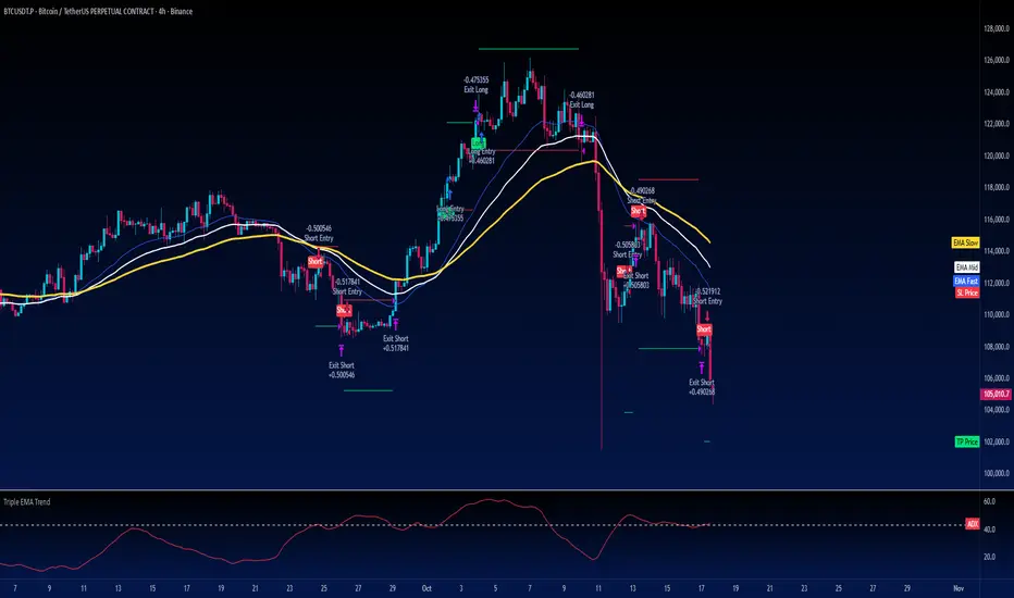
Turtle Strategy - Triple EMA Trend with ADX and ATRDescription
The Triple EMA Trend strategy is a directional momentum system built on the alignment of three exponential moving averages and a strong ADX confirmation filter. It is designed to capture established trends while maintaining disciplined risk management through ATR-based stops and targets.
Core Logic
The system activates only under high-trend conditions, defined by the Average Directional Index (ADX) exceeding a configurable threshold (default: 43).
A bullish setup occurs when the short-term EMA is above the mid-term EMA, which in turn is above the long-term EMA, and price trades above the fastest EMA.
A bearish setup is the mirror condition.
Execution Rules
Entry:
• Long when ADX confirms trend strength and EMA alignment is bullish.
• Short when ADX confirms trend strength and EMA alignment is bearish.
Exit:
• Stop Loss: 1.8 × ATR below (for longs) or above (for shorts) the entry price.
• Take Profit: 3.3 × ATR in the direction of the trade.
Both parameters are configurable.
Additional Features
• Start/end date inputs for controlled backtesting.
• Selective activation of long or short trades.
• Built-in commission and position sizing (percent of equity).
• Full visual representation of EMAs, ADX, stop-loss, and target levels.
This strategy emphasizes clean trend participation, strict entry qualification, and consistent reward-to-risk structure. Ideal for swing or medium-term testing across trending assets.
Seasonality Heatmap [QuantAlgo]🟢 Overview
The Seasonality Heatmap analyzes years of historical data to reveal which months and weekdays have consistently produced gains or losses, displaying results through color-coded tables with statistical metrics like consistency scores (1-10 rating) and positive occurrence rates. By calculating average returns for each calendar month and day-of-week combination, it identifies recognizable seasonal patterns (such as which months or weekdays tend to rally versus decline) and synthesizes this into actionable buy low/sell high timing possibilities for strategic entries and exits. This helps traders and investors spot high-probability seasonal windows where assets have historically shown strength or weakness, enabling them to align positions with recurring bull and bear market patterns.
🟢 How It Works
1. Monthly Heatmap
How % Return is Calculated:
The indicator fetches monthly closing prices (or Open/High/Low based on user selection) and calculates the percentage change from the previous month:
(Current Month Price - Previous Month Price) / Previous Month Price × 100
Each cell in the heatmap represents one month's return in a specific year, creating a multi-year historical view
Colors indicate performance intensity: greener/brighter shades for higher positive returns, redder/brighter shades for larger negative returns
What Averages Mean:
The "Avg %" row displays the arithmetic mean of all historical returns for each calendar month (e.g., averaging all Januaries together, all Februaries together, etc.)
This metric identifies historically recurring patterns by showing which months have tended to rise or fall on average
Positive averages indicate months that have typically trended upward; negative averages indicate historically weaker months
Example: If April shows +18.56% average, it means April has averaged a 18.56% gain across all years analyzed
What Months Up % Mean:
Shows the percentage of historical occurrences where that month had a positive return (closed higher than the previous month)
Calculated as:
(Number of Months with Positive Returns / Total Months) × 100
Values above 50% indicate the month has been positive more often than negative; below 50% indicates more frequent negative months
Example: If October shows "64%", then 64% of all historical Octobers had positive returns
What Consistency Score Means:
A 1-10 rating that measures how predictable and stable a month's returns have been
Calculated using the coefficient of variation (standard deviation / mean) - lower variation = higher consistency
High scores (8-10, green): The month has shown relatively stable behavior with similar outcomes year-to-year
Medium scores (5-7, gray): Moderate consistency with some variability
Low scores (1-4, red): High variability with unpredictable behavior across different years
Example: A consistency score of 8/10 indicates the month has exhibited recognizable patterns with relatively low deviation
What Best Means:
Shows the highest percentage return achieved for that specific month, along with the year it occurred
Reveals the maximum observed upside and identifies outlier years with exceptional performance
Useful for understanding the range of possible outcomes beyond the average
Example: "Best: 2016: +131.90%" means the strongest January in the dataset was in 2016 with an 131.90% gain
What Worst Means:
Shows the most negative percentage return for that specific month, along with the year it occurred
Reveals maximum observed downside and helps understand the range of historical outcomes
Important for risk assessment even in months with positive averages
Example: "Worst: 2022: -26.86%" means the weakest January in the dataset was in 2022 with a 26.86% loss
2. Day-of-Week Heatmap
How % Return is Calculated:
Calculates the percentage change from the previous day's close to the current day's price (based on user's price source selection)
Returns are aggregated by day of the week within each calendar month (e.g., all Mondays in January, all Tuesdays in January, etc.)
Each cell shows the average performance for that specific day-month combination across all historical data
Formula:
(Current Day Price - Previous Day Close) / Previous Day Close × 100
What Averages Mean:
The "Avg %" row at the bottom aggregates all months together to show the overall average return for each weekday
Identifies broad weekly patterns across the entire dataset
Calculated by summing all daily returns for that weekday across all months and dividing by total observations
Example: If Monday shows +0.04%, Mondays have averaged a 0.04% change across all months in the dataset
What Days Up % Mean:
Shows the percentage of historical occurrences where that weekday had a positive return
Calculated as:
(Number of Positive Days / Total Days Observed) × 100
Values above 50% indicate the day has been positive more often than negative; below 50% indicates more frequent negative days
Example: If Fridays show "54%", then 54% of all Fridays in the dataset had positive returns
What Consistency Score Means:
A 1-10 rating measuring how stable that weekday's performance has been across different months
Based on the coefficient of variation of daily returns for that weekday across all 12 months
High scores (8-10, green): The weekday has shown relatively consistent behavior month-to-month
Medium scores (5-7, gray): Moderate consistency with some month-to-month variation
Low scores (1-4, red): High variability across months, with behavior differing significantly by calendar month
Example: A consistency score of 7/10 for Wednesdays means they have performed with moderate consistency throughout the year
What Best Means:
Shows which calendar month had the strongest average performance for that specific weekday
Identifies favorable day-month combinations based on historical data
Format shows the month abbreviation and the average return achieved
Example: "Best: Oct: +0.20%" means Mondays averaged +0.20% during October months in the dataset
What Worst Means:
Shows which calendar month had the weakest average performance for that specific weekday
Identifies historically challenging day-month combinations
Useful for understanding which month-weekday pairings have shown weaker performance
Example: "Worst: Sep: -0.35%" means Tuesdays averaged -0.35% during September months in the dataset
3. Optimal Timing Table/Summary Table
→ Best Month to BUY: Identifies the month with the lowest average return (most negative or least positive historically), representing periods where prices have historically been relatively lower
Based on the observation that buying during historically weaker months may position for subsequent recovery
Shows the month name, its average return, and color-coded performance
Example: If May shows -0.86% as "Best Month to BUY", it means May has historically averaged -0.86% in the analyzed period
→ Best Month to SELL: Identifies the month with the highest average return (most positive historically), representing periods where prices have historically been relatively higher
Based on historical strength patterns in that month
Example: If July shows +1.42% as "Best Month to SELL", it means July has historically averaged +1.42% gains
→ 2nd Best Month to BUY: The second-lowest performing month based on average returns
Provides an alternative timing option based on historical patterns
Offers flexibility for staged entries or when the primary month doesn't align with strategy
Example: Identifies the next-most favorable historical buying period
→ 2nd Best Month to SELL: The second-highest performing month based on average returns
Provides an alternative exit timing based on historical data
Useful for staged profit-taking or multiple exit opportunities
Identifies the secondary historical strength period
Note: The same logic applies to "Best Day to BUY/SELL" and "2nd Best Day to BUY/SELL" rows, which identify weekdays based on average daily performance across all months. Days with lowest averages are marked as buying opportunities (historically weaker days), while days with highest averages are marked for selling (historically stronger days).
🟢 Examples
Example 1: NVIDIA NASDAQ:NVDA - Strong May Pattern with High Consistency
Analyzing NVIDIA from 2015 onwards, the Monthly Heatmap reveals May averaging +15.84% with 82% of months being positive and a consistency score of 8/10 (green). December shows -1.69% average with only 40% of months positive and a low 1/10 consistency score (red). The Optimal Timing table identifies December as "Best Month to BUY" and May as "Best Month to SELL." A trader recognizes this high-probability May strength pattern and considers entering positions in late December when prices have historically been weaker, then taking profits in May when the seasonal tailwind typically peaks. The high consistency score in May (8/10) provides additional confidence that this pattern has been relatively stable year-over-year.
Example 2: Crypto Market Cap CRYPTOCAP:TOTALES - October Rally Pattern
An investor examining total crypto market capitalization notices September averaging -2.42% with 45% of months positive and 5/10 consistency, while October shows a dramatic shift with +16.69% average, 90% of months positive, and an exceptional 9/10 consistency score (blue). The Day-of-Week heatmap reveals Mondays averaging +0.40% with 54% positive days and 9/10 consistency (blue), while Thursdays show only +0.08% with 1/10 consistency (yellow). The investor uses this multi-layered analysis to develop a strategy: enter crypto positions on Thursdays during late September (combining the historically weak month with the less consistent weekday), then hold through October's historically strong period, considering exits on Mondays when intraweek strength has been most consistent.
Example 3: Solana BINANCE:SOLUSDT - Extreme January Seasonality
A cryptocurrency trader analyzing Solana observes an extraordinary January pattern: +59.57% average return with 60% of months positive and 8/10 consistency (teal), while May shows -9.75% average with only 33% of months positive and 6/10 consistency. August also displays strength at +59.50% average with 7/10 consistency. The Optimal Timing table confirms May as "Best Month to BUY" and January as "Best Month to SELL." The Day-of-Week data shows Sundays averaging +0.77% with 8/10 consistency (teal). The trader develops a seasonal rotation strategy: accumulate SOL positions during May weakness, hold through the historically strong January period (which has shown this extreme pattern with reasonable consistency), and specifically target Sunday exits when the weekday data shows the most recognizable strength pattern.

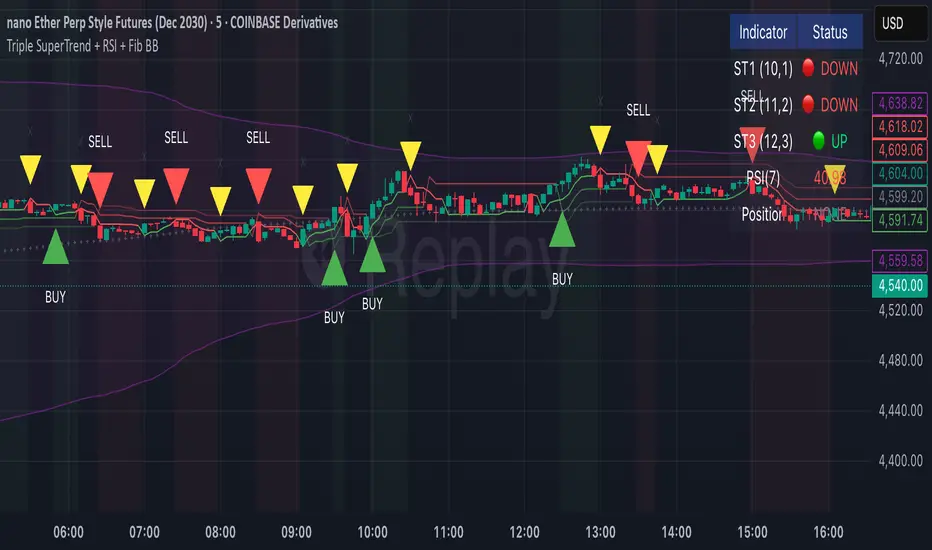
Triple SuperTrend + RSI + Fib BBTriple SuperTrend + RSI + Fibonacci Bollinger Bands Strategy
📊 Overview
This advanced trading strategy combines the power of three SuperTrend indicators with RSI confirmation and Fibonacci Bollinger Bands to generate high-probability trade signals. The strategy is designed to capture strong trending moves while filtering out false signals through multi-indicator confluence.
🔧 Core Components
Three SuperTrend Indicators
The strategy uses three SuperTrend indicators with progressively longer periods and multipliers:
SuperTrend 1: 10-period ATR, 1.0 multiplier (fastest, most sensitive)
SuperTrend 2: 11-period ATR, 2.0 multiplier (medium sensitivity)
SuperTrend 3: 12-period ATR, 3.0 multiplier (slowest, most stable)
This layered approach ensures that all three timeframe perspectives align before generating a signal, significantly reducing false entries.
RSI Confirmation (7-period)
The Relative Strength Index acts as a momentum filter:
Long signals require RSI > 50 (bullish momentum)
Short signals require RSI < 50 (bearish momentum)
This prevents entries during weak or divergent price action.
Fibonacci Bollinger Bands (200, 2.618)
Uses a 200-period Simple Moving Average with 2.618 standard deviation bands (Fibonacci ratio). These bands serve dual purposes:
Visual representation of price extremes
Automatic exit trigger when price reaches overextended levels
📈 Entry Logic
LONG Entry (BUY Signal)
A LONG position is opened when ALL of the following conditions are met simultaneously:
All three SuperTrend indicators turn green (bullish)
RSI(7) is above 50
This is the first bar where all conditions align (no repainting)
SHORT Entry (SELL Signal)
A SHORT position is opened when ALL of the following conditions are met simultaneously:
All three SuperTrend indicators turn red (bearish)
RSI(7) is below 50
This is the first bar where all conditions align (no repainting)
🚪 Exit Logic
Positions are automatically closed when ANY of these conditions occur:
SuperTrend Color Change: Any one of the three SuperTrend indicators changes direction
Fibonacci BB Touch: Price reaches or exceeds the upper or lower Fibonacci Bollinger Band (2.618 standard deviations)
This dual-exit approach protects profits by:
Exiting quickly when trend momentum shifts (SuperTrend change)
Taking profits at statistical price extremes (Fib BB touch)
🎨 Visual Features
Signal Arrows
Green Up Arrow (BUY): Appears below the bar when long entry conditions are met
Red Down Arrow (SELL): Appears above the bar when short entry conditions are met
Yellow Down Arrow (EXIT): Appears above the bar when exit conditions are met
Background Coloring
Light Green Tint: All three SuperTrends are bullish (uptrend environment)
Light Red Tint: All three SuperTrends are bearish (downtrend environment)
SuperTrend Lines
Three colored lines plotted with varying opacity:
Solid line (ST1): Most responsive to price changes
Semi-transparent (ST2): Medium-term trend
Most transparent (ST3): Long-term trend structure
Dashboard
Real-time information panel showing:
Individual SuperTrend status (UP/DOWN)
Current RSI value and color-coded status
Current position (LONG/SHORT/FLAT)
Net Profit/Loss
⚙️ Customizable Parameters
SuperTrend Settings
ATR periods for each SuperTrend (default: 10, 11, 12)
Multipliers for each SuperTrend (default: 1.0, 2.0, 3.0)
RSI Settings
RSI length (default: 7)
RSI source (default: close)
Fibonacci Bollinger Bands
BB length (default: 200)
BB multiplier (default: 2.618)
Strategy Options
Enable/disable long trades
Enable/disable short trades
Initial capital
Position sizing
Commission settings
💡 Strategy Philosophy
This strategy is built on the principle of confluence trading - waiting for multiple independent indicators to align before taking a position. By requiring three SuperTrend indicators AND RSI confirmation, the strategy filters out the majority of low-probability setups.
The multi-timeframe SuperTrend approach ensures that short-term, medium-term, and longer-term trends are all in agreement, which typically occurs during strong, sustainable price moves.
The exit strategy is equally important, using both trend-following logic (SuperTrend changes) and mean-reversion logic (Fibonacci BB touches) to adapt to different market conditions.
📊 Best Use Cases
Trending Markets: Works best in markets with clear directional bias
Higher Timeframes: Designed for 15-minute to daily charts
Volatile Assets: SuperTrend indicators excel in assets with clear trends
Swing Trading: Hold times typically range from hours to days
⚠️ Important Notes
No Repainting: All signals are confirmed and will not change on historical bars
One Signal Per Setup: The strategy prevents duplicate signals on consecutive bars
Exit Protection: Always exits before potentially taking an opposite position
Visual Clarity: All three SuperTrend lines are visible simultaneously for transparency
🎯 Recommended Settings
While default parameters are optimized for general use, consider:
Crypto/Volatile Markets: May benefit from slightly higher multipliers
Forex: Default settings work well for major pairs
Stocks: Consider longer BB periods (250-300) for daily charts
Lower Timeframes: Reduce all periods proportionally for scalping
📝 Alerts
Built-in alert conditions for:
BUY signal triggered
SELL signal triggered
EXIT signal triggered
Set up notifications to never miss a trade opportunity!
Disclaimer: This strategy is for educational and informational purposes only. Past performance does not guarantee future results. Always backtest thoroughly and practice proper risk management before live trading.
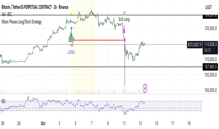
Moon Phases Long/Short StrategyThis is an experiment of Moon Phases, likely buy when full moon and sell when new moon with few changes, like it would buy a day ahead or sometimes sell a day post these events, with Stop loss and take profits, 50% profitable so sounds good to me
Long only good for bitcoin gold, both modes(L+S) better for stocks and alt coins
Adaptive Trend Breaks Adaptive Trend Breaks
## WHAT IT DOES
This script is a modified and enhanced version of "Trendline Breakouts With Targets" concept by ChartPrime.
Adaptive Trend Breaks (ATB) is a trendline breakout system optimized for scalping liquid futures contracts. The indicator automatically draws dynamic support and resistance trendlines based on pivot points, then generates trade signals when price breaks through these levels with confirmation filters. It includes automated target and stop-loss placement with real-time P&L tracking in dollars.
## HOW IT WORKS
**Trendline Detection Method:**
The indicator uses pivot high/low detection to identify significant price turning points. When a new pivot forms, it calculates the slope between consecutive pivots to draw dynamic trendlines. These lines extend forward based on the established trend angle, creating actionable support and resistance zones.
**Band System:**
Around each trendline, the script creates a "band" using a volatility-adjusted calculation: `ATR(14) * 0.2 * bandwidth multiplier / 2`. This adaptive band accounts for current market conditions - wider during volatile periods, tighter during quiet markets.
**Breakout Logic:**
A breakout signal triggers when:
1. Price closes beyond the trendline + band zone
2. Volume exceeds the 20-period moving average by your set multiplier (default 1.2x)
3. Price is within Regular Trading Hours (9:30-16:00 EST) if session filter enabled
4. Current ATR meets minimum volatility threshold (prevents trading dead markets)
**Target & Stop Calculation:**
Upon breakout confirmation:
- **Entry**: Trendline breach point
- **Target**: Entry ± (bandwidth × target multiplier) - default 8x for quick scalps
- **Stop**: Entry ± (bandwidth × stop multiplier) - default 8x for 1:1 risk/reward
- Multipliers adjust automatically to market volatility through the ATR-based band
**P&L Conversion:**
The script converts point movements to dollars using:
```
Dollar P&L = (Price Points × Contract Point Value × Quantity)
```
For example, a 10-point NQ move with 2 contracts = 10 × $20 × 2 = $400
## HOW TO USE IT
**Setup:**
1. Select your instrument (NQ/ES/YM/RTY) - point values auto-configure
2. Set contract quantity for accurate dollar P&L
3. Choose pivot period (lower = more signals but more noise, default 5 for scalping)
4. Adjust bandwidth multiplier if trendlines are too tight/loose (1-5 range)
**Filters Configuration:**
- **Volume Filter**: Requires breakout volume > moving average × multiplier. Increase multiplier (1.5-2.0) for higher conviction trades
- **Session Filter**: Enable to trade only RTH. Disable for 24-hour trading
- **ATR Filter**: Prevents signals during low volatility. Increase minimum % for more active markets only
**Risk Management:**
- Set target/stop multipliers based on your risk tolerance
- 8x bandwidth = approximately 1:1 risk/reward for most liquid futures
- Enable trailing stops for trend-following approach (moves stop to protect profits)
- Adjust line length to see targets further into the future
**Statistics Table:**
- Choose timeframe to analyze: all-time, today, this week, custom days
- Monitor win rate, profit factor, and net P&L in dollars
- Track long vs short performance separately
- See real-time unrealized P&L on active trades
**Reading Signals:**
- **Green triangle below bar** = Long breakout (resistance broken)
- **Red triangle above bar** = Short breakout (support broken)
- **White dashed line** = Entry price
- **Orange line** = Take profit target with dollar value
- **Red line** = Stop loss with dollar value
- **Green checkmark (✓)** = Target hit, winning trade
- **Red X (✗)** = Stop hit, losing trade
## WHAT IT DOES NOT DO
**Limitations to Understand:**
- Does not predict future trendline formations - it reacts to breakouts after they occur
- Historical trendlines disappear after breakout (not kept on chart for clarity)
- Requires sufficient volatility - may not signal in extremely quiet markets
- Volume filter requires exchange volume data (not available on all symbols)
- Statistics are indicator-based simulations, not actual trading results
- Does not account for slippage, commissions, or order fills
## BEST PRACTICES
**Recommended Settings by Market:**
- **NQ (Nasdaq)**: Default settings work well, consider volume multiplier 1.3-1.5
- **ES (S&P 500)**: Slightly slower, try period 7-8, volume 1.2
- **YM (Dow)**: Lower volatility, reduce bandwidth to 1.5-2
- **RTY (Russell)**: Higher volatility, increase bandwidth to 3-4
**Risk Management:**
- Never risk more than 2-3% of account per trade
- Use contract quantity calculator: Max Risk $ ÷ (Stop Distance × Point Value)
- Start with 1 contract while learning the system
- Backtest your specific timeframe and instrument before live trading
**Optimization Tips:**
- Increase pivot period (7-10) for fewer but higher-quality signals
- Raise volume multiplier (1.5-2.0) in choppy markets
- Lower target/stop multipliers (5-6x) for tighter profit taking
- Use trailing stops in strong trending conditions
- Disable session filter for overnight gaps and Asia session moves
## TECHNICAL DETAILS
**Key Calculations:**
- Pivot Detection: `ta.pivothigh(high, period, period/2)` and `ta.pivotlow(low, period, period/2)`
- Slope Calculation: `(newPivot - oldPivot) / (newTime - oldTime)`
- Adaptive Band: `min(ATR(14) * 0.2, close * 0.002) * multiplier / 2`
- Breakout Confirmation: Price crosses trendline + 10% of band threshold
**Data Requirements:**
- Minimum bars in view: 500 for proper pivot calculation
- Volume data required for volume filter accuracy
- Intraday timeframes recommended (1min - 15min) for scalping
- Works on any timeframe but optimized for fast execution
**Performance Metrics:**
All statistics calculate based on indicator signals:
- Tracks every signal as a trade from entry to TP/SL
- P&L in actual contract dollar values
- Win rate = (Winning trades / Total trades) × 100
- Profit factor = Gross profit / Gross loss
- Separates long/short performance for bias analysis
## IDEAL FOR
- Futures scalpers and day traders
- Traders who prefer visual trendline breakouts
- Those wanting automated TP/SL placement
- Traders tracking performance in dollar terms
- Multiple timeframe analysis (compare 1min vs 5min signals)
## NOT SUITABLE FOR
- Swing trading (targets too close)
- Stocks/forex without modifying point values
- Extremely low timeframes (<30 seconds) - too much noise
- Markets without volume data if using volume filter
- Illiquid contracts (signals may not execute at shown prices)
---
**Settings Summary:**
- Core: Period, bandwidth, extension, trendline style
- Filters: Volume, RTH session, ATR volatility
- Risk: R:R ratio, target/stop multipliers, trailing stop
- Display: Stats table position, size, colors
- Stats: Timeframe selection (all-time to custom days)
**License:** This indicator is published open-source under Mozilla Public License 2.0. You may use and modify the code with proper attribution.
**Disclaimer:** This indicator is for educational purposes. Past performance does not guarantee future results. Always practice proper risk management and test thoroughly before live trading.
---
## CREDITS & ATTRIBUTION
This script builds upon the "Trendline Breakouts With Targets" concept by ChartPrime with significant enhancements:
**Major Improvements Added:**
- **Futures-Specific Calculations**: Automated dollar P&L conversion using actual contract point values (NQ=$20, ES=$50, YM=$5, RTY=$50)
- **Advanced Statistics Engine**: Comprehensive performance tracking with customizable timeframe analysis (today, week, month, custom ranges)
- **Multi-Layer Filtering System**: Volume confirmation, RTH session filter, and ATR volatility filter to reduce false signals
- **Professional Trade Management**: Enhanced visual trade tracking with separate TP/SL lines, dollar value labels, and optional trailing stops
- **Optimized for Scalping**: Faster pivot periods (5 vs 10), tighter bands, and reduced extension bars for quick entries
Original trendline detection methodology by ChartPrime - used with modification under Mozilla Public License 2.0.
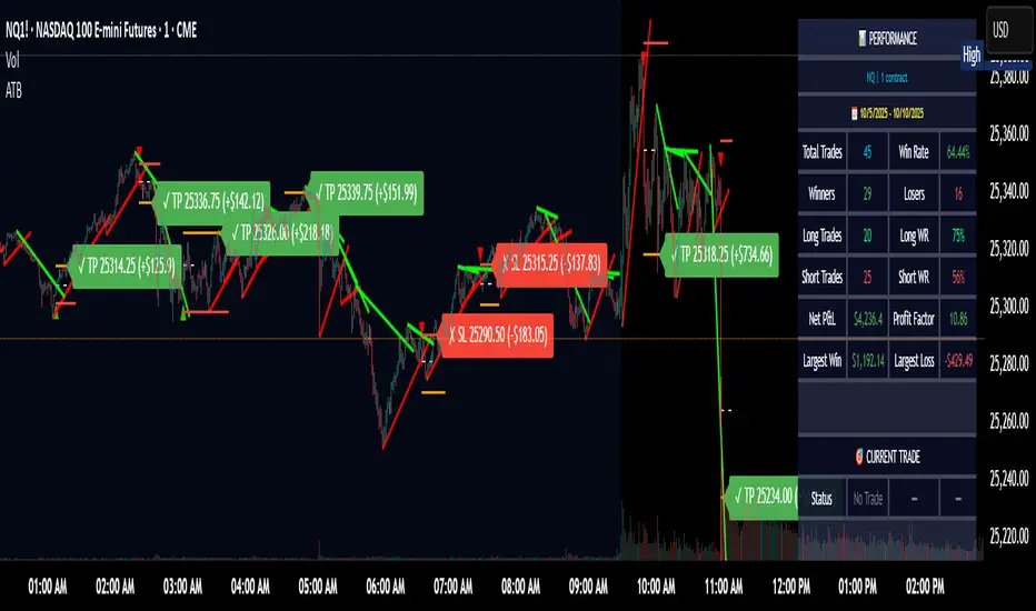
Larry Williams Oops StrategyThis strategy is a modern take on Larry Williams’ classic Oops setup. It trades intraday while referencing daily bars to detect opening gaps and align entries with the prior day’s direction. Risk is managed with day-based stops, and—unlike the original—all positions are closed at the end of the session (or at the last bar’s close), not at a fixed profit target or the first profitable open.
Entry Rules
Long setup (bullish reversion): Today opens below yesterday’s low (down gap) and yesterday’s candle was bearish. Place a buy stop at yesterday’s low + Filter (ticks).
Short setup (bearish reversion): Today opens above yesterday’s high (up gap) and yesterday’s candle was bullish. Place a sell stop at yesterday’s high − Filter (ticks).
Longs are only taken on down-gap days; shorts only on up-gap days.
Protective Stop
If long, stop loss trails the current day’s low.
If short, stop loss trails the current day’s high.
Exit Logic
Positions are force-closed at the end of the session (in the last bar), ensuring no overnight exposure. There is no take-profit; only stop loss or end-of-day flat.
Notes
This strategy is designed for intraday charts (minutes/seconds) using daily data for gaps and prior-day direction.
Longs/shorts can be enabled or disabled independently.

MNQ TopStep 50K | Ultra Quality v3.0MNQ TopStep 50K | Ultra Quality v3.0 - Publish Summary
📊 Overview
A professional-grade trading indicator designed specifically for MNQ futures traders using TopStep funded accounts. Combines 7 technical confirmations with 5 advanced safety filters to deliver high-quality trade signals while managing drawdown risk.
🎯 Key Features
Core Signal System
7-Point Confirmation: VWAP, EMA crossovers, 15-min HTF trend, MACD, RSI, ADX, and Volume
Signal Grading: Each signal is rated A+ through D based on 7 quality factors
Quality Threshold: Adjustable minimum grade requirement (A+, A, B, C, D)
Advanced Safety Filters (Customizable)
Mean Reversion Filter - Prevents chasing extended moves beyond VWAP bands
ATR Spike Filter - Avoids trading during extreme volatility events
EMA Spacing Filter - Ensures proper trend separation (optional)
Momentum Filter - Requires consecutive directional bars (optional)
Multi-Timeframe Confirmation - Aligns with 15-min trend (optional)
TopStep Risk Management
Real-time drawdown tracking
Position sizing calculator based on remaining cushion
Daily loss limit monitoring
Consecutive loss protection
Max trades per day limiter
Visual Components
VWAP with 1σ, 2σ, 3σ bands
EMA 9/21 with cloud fill
15-min EMA 50 for HTF trend
Comprehensive metrics dashboard
Risk management panel
Filter status panel
Detailed trade labels with entry, stops, and targets
⚙️ Default Settings (Balanced for Regular Signals)
Technical Indicators
Fast EMA: 9 | Slow EMA: 21 | HTF EMA: 50 (15-min)
MACD: 10/22/9
RSI: 14 period | Thresholds: 52 (buy) / 48 (sell)
ADX: 14 period | Minimum: 20
ATR: 14 period | Stop: 2x | TP1: 2x | TP2: 3x
Volume: 1.2x average required
Session Settings
Default: 9:30 AM - 11:30 AM ET (adjustable)
Avoids first 15 minutes after market open
Customizable trading hours
Safety Filters (Default Configuration)
✅ Mean Reversion: Enabled (2.5σ max from VWAP)
✅ ATR Spike: Enabled (2.0x threshold)
❌ EMA Spacing: Disabled (can enable for quality)
❌ Momentum: Disabled (can enable for quality)
❌ MTF Confirmation: Disabled (can enable for quality)
Risk Controls
Minimum Signal Quality: C (adjustable to A+ for fewer/better signals)
Min Bars Between Signals: 10
Max Trades Per Day: 5
Stop After Consecutive Losses: 2
📈 Expected Performance
With Default Settings:
Signals per week: 10-15 trades
Estimated win rate: 55-60%
Risk-Reward: 1:2 (TP1) and 1:3 (TP2)
With Aggressive Settings (Min Quality = D, All Filters Off):
Signals per week: 20-25 trades
Estimated win rate: 50-55%
With Conservative Settings (Min Quality = A, All Filters On):
Signals per week: 3-5 trades
Estimated win rate: 65-70%
🚀 How to Use
Basic Setup:
Add indicator to MNQ 5-minute chart
Adjust TopStep account settings in inputs
Set your risk per trade percentage (default: 0.5%)
Configure trading session hours
Set minimum signal quality (Start with C for balanced results)
Signal Interpretation:
Green Triangle (BUY): Long signal - all confirmations aligned
Red Triangle (SELL): Short signal - all confirmations aligned
Label Details: Shows entry, stop loss, take profit levels, position size, and signal grade
Signal Grade: A+ = Elite (6-7 points) | A = Strong (5) | B = Good (4) | C = Fair (3)
Dashboard Monitoring:
Top Right: Technical metrics and market conditions
Top Left: Filter status (which filters are passing/blocking)
Bottom Right: TopStep risk metrics and position sizing
⚡ Customization Tips
For More Signals:
Lower "Minimum Signal Quality" to D
Decrease ADX threshold to 18-20
Lower RSI thresholds to 50/50
Reduce Volume multiplier to 1.1x
Disable additional filters
For Higher Quality (Fewer Signals):
Raise "Minimum Signal Quality" to A or A+
Increase ADX threshold to 25-30
Enable all 5 advanced filters
Tighten VWAP distance to 2.0σ
Increase momentum requirement to 3-4 bars
For TopStep Compliance:
Adjust "Max Total Drawdown" and "Daily Loss Limit" to match your account
Update "Already Used Drawdown" daily
Monitor the Risk Panel for cushion remaining
Use recommended contract sizing
🛡️ Risk Disclaimer
IMPORTANT: This indicator is for educational and informational purposes only.
Past performance does not guarantee future results
All trading involves substantial risk of loss
Use proper risk management and position sizing
Test thoroughly in paper trading before live use
The indicator does not guarantee profitable trades
Adjust settings based on your risk tolerance and trading style
Always comply with your broker's and TopStep's rules
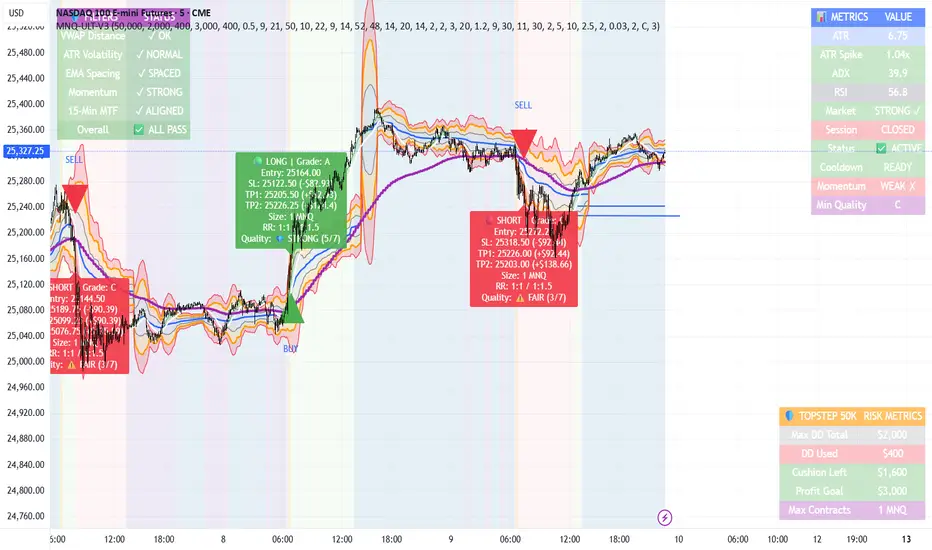
MNQ TopStep 50K | Ultra Quality v3.0MNQ TopStep 50K | Ultra Quality v3.0 - Publish Summary📊 OverviewA professional-grade trading indicator designed specifically for MNQ futures traders using TopStep funded accounts. Combines 7 technical confirmations with 5 advanced safety filters to deliver high-quality trade signals while managing drawdown risk.🎯 Key FeaturesCore Signal System
7-Point Confirmation: VWAP, EMA crossovers, 15-min HTF trend, MACD, RSI, ADX, and Volume
Signal Grading: Each signal is rated A+ through D based on 7 quality factors
Quality Threshold: Adjustable minimum grade requirement (A+, A, B, C, D)
Advanced Safety Filters (Customizable)
Mean Reversion Filter - Prevents chasing extended moves beyond VWAP bands
ATR Spike Filter - Avoids trading during extreme volatility events
EMA Spacing Filter - Ensures proper trend separation (optional)
Momentum Filter - Requires consecutive directional bars (optional)
Multi-Timeframe Confirmation - Aligns with 15-min trend (optional)
TopStep Risk Management
Real-time drawdown tracking
Position sizing calculator based on remaining cushion
Daily loss limit monitoring
Consecutive loss protection
Max trades per day limiter
Visual Components
VWAP with 1σ, 2σ, 3σ bands
EMA 9/21 with cloud fill
15-min EMA 50 for HTF trend
Comprehensive metrics dashboard
Risk management panel
Filter status panel
Detailed trade labels with entry, stops, and targets
⚙️ Default Settings (Balanced for Regular Signals)Technical Indicators
Fast EMA: 9 | Slow EMA: 21 | HTF EMA: 50 (15-min)
MACD: 10/22/9
RSI: 14 period | Thresholds: 52 (buy) / 48 (sell)
ADX: 14 period | Minimum: 20
ATR: 14 period | Stop: 2x | TP1: 2x | TP2: 3x
Volume: 1.2x average required
Session Settings
Default: 9:30 AM - 11:30 AM ET (adjustable)
Avoids first 15 minutes after market open
Customizable trading hours
Safety Filters (Default Configuration)
✅ Mean Reversion: Enabled (2.5σ max from VWAP)
✅ ATR Spike: Enabled (2.0x threshold)
❌ EMA Spacing: Disabled (can enable for quality)
❌ Momentum: Disabled (can enable for quality)
❌ MTF Confirmation: Disabled (can enable for quality)
Risk Controls
Minimum Signal Quality: C (adjustable to A+ for fewer/better signals)
Min Bars Between Signals: 10
Max Trades Per Day: 5
Stop After Consecutive Losses: 2
📈 Expected PerformanceWith Default Settings:
Signals per week: 10-15 trades
Estimated win rate: 55-60%
Risk-Reward: 1:2 (TP1) and 1:3 (TP2)
With Aggressive Settings (Min Quality = D, All Filters Off):
Signals per week: 20-25 trades
Estimated win rate: 50-55%
With Conservative Settings (Min Quality = A, All Filters On):
Signals per week: 3-5 trades
Estimated win rate: 65-70%
🚀 How to UseBasic Setup:
Add indicator to MNQ 5-minute chart
Adjust TopStep account settings in inputs
Set your risk per trade percentage (default: 0.5%)
Configure trading session hours
Set minimum signal quality (Start with C for balanced results)
Signal Interpretation:
Green Triangle (BUY): Long signal - all confirmations aligned
Red Triangle (SELL): Short signal - all confirmations aligned
Label Details: Shows entry, stop loss, take profit levels, position size, and signal grade
Signal Grade: A+ = Elite (6-7 points) | A = Strong (5) | B = Good (4) | C = Fair (3)
Dashboard Monitoring:
Top Right: Technical metrics and market conditions
Top Left: Filter status (which filters are passing/blocking)
Bottom Right: TopStep risk metrics and position sizing
⚡ Customization TipsFor More Signals:
Lower "Minimum Signal Quality" to D
Decrease ADX threshold to 18-20
Lower RSI thresholds to 50/50
Reduce Volume multiplier to 1.1x
Disable additional filters
For Higher Quality (Fewer Signals):
Raise "Minimum Signal Quality" to A or A+
Increase ADX threshold to 25-30
Enable all 5 advanced filters
Tighten VWAP distance to 2.0σ
Increase momentum requirement to 3-4 bars
For TopStep Compliance:
Adjust "Max Total Drawdown" and "Daily Loss Limit" to match your account
Update "Already Used Drawdown" daily
Monitor the Risk Panel for cushion remaining
Use recommended contract sizing
🛡️ Risk DisclaimerIMPORTANT: This indicator is for educational and informational purposes only.
Past performance does not guarantee future results
All trading involves substantial risk of loss
Use proper risk management and position sizing
Test thoroughly in paper trading before live use
The indicator does not guarantee profitable trades
Adjust settings based on your risk tolerance and trading style
Always comply with your broker's and TopStep's rules

Alt buy signal 1H Entry + 4H Confirm (MACD + Stoch RSI + HMA)This indicator is a multi-timeframe (MTF) analysis tool designed for the ALT trading , capturing entry signals on the 1-hour (1H) timeframe and confirming trends on the 4-hour (4H) timeframe. It combines MACD, Stoch RSI, and Hull Moving Average (HMA) to identify precise buy opportunities, particularly at reversal points after a downtrend or during trend shifts. It visually marks both past and current BUY signals for easy reference.
Key Features:
1H Entry Signal (Early Ping): Triggers on a MACD golden cross (below 0) combined with a Stoch RSI oversold cross (below 20), offering an initial buy opportunity.
4H Trend Confirmation (Entry Ready): Validates the trend with a 4H MACD histogram rising (in negative territory) or a golden cross, plus a Stoch RSI turn-up (above 30).
Past BUY Display: Labels past data points where these conditions were met as "1H BUY" or "FULL BUY," facilitating backtesting.
HMA Filter: Optional HMA(16) to confirm price breakouts, enhancing trend validation.
Purpose: Ideal for short-term scalping and swing trading. Supports a two-step strategy: initial partial entry on 1H signals, followed by additional entry on 4H confirmation.
Usage Instructions
Installation: Add the indicator to an IMX/USDT 1H chart on TradingView.
Signal Interpretation:
lime "1H BUY": 1H conditions met, consider initial entry (stop-loss: 3-5% below recent low).
green "FULL BUY": 1H+4H conditions met, confirm trend for additional entry (take-profit: 10% below recent swing high).
Customization: Adjust TF (1H/4H), MACD/Stoch RSI parameters, and HMA usage via the input settings.
Alert Setup: Enable alerts for "ENTRY READY" (1H+4H) or "EARLY PING" (1H only) conditions.
Advantages
Accuracy: Reduces false signals by combining MACD golden cross below 0 with Stoch RSI oversold conditions.
Dual Confirmation: 1H for quick timing and 4H for trend validation, improving risk management.
Visualization: Past BUY points enable easy backtesting and pattern recognition.
Flexibility: 4H confirmation mode adjustable (histogram rise or golden cross).
Limitations
Timeframe Dependency: Optimized for 1H charts; may not work on other timeframes.
Market Conditions: Potential whipsaws in sideways markets; additional filters (e.g., RSI > 50) recommended.
Manual Management: Stop-loss and take-profit require user discretion.

my_strategy_2.0Overview:
This is a high-speed scalping strategy optimized for volatile crypto assets (BTC, ETH, etc.) on timeframes 1m–5m. It combines trend-following SuperTrend with confirmations from MACD, RSI, Bollinger Bands, and volume spikes for precise entries. Focus on quick profits (1–3 ATR) with strict risk control: partial take-profits, stop-loss, and trailing breakeven after the first TP.
Key Signals:
Long: SuperTrend flip up + MACD crossover up + RSI >50 + BB Upper breakout + volume spike + volatility filter (ATR >0.5%).
Short: Similar but downward.
Exits and Risks:
TP: 33% at +1 ATR, 33% at +2 ATR, 34% at +3 ATR (customizable).
SL: Initial at -1 ATR, after TP1 — to breakeven with trailing on BB midline (optional).
Filters: Minimum ATR to avoid flat markets; realistic commissions in backtests.
Recommendations:
Test on 2020–2025 data (out-of-sample 2024+). Expected Win Rate ~55%, Profit Factor >1.8, Drawdown <10%. Ideal for 1–2% risk per trade. Not for beginners — use paper trading.
Disclaimer: Past results do not guarantee future performance. Trade at your own risk.
(Pine v6 code, ready for publication. Author: gopog777 with expert fixes.)
DTM 444 BANDS 🚀DTM 444 BANDS 🚀:
The DTM 444 BANDS 🚀 is a powerful, multi-purpose trading indicator combining Supertrend, Dynamic Band Levels, Breakout Signals, and Volume Confirmation to help traders identify high-probability trade setups across different timeframes.
🔧 Key Features
✅ Multi-Timeframe Support
Analyze price action across any timeframe using the Timeframe input.
All band calculations (High, Low, Midline, and Supertrend) are pulled from a higher timeframe for clearer context.
✅ Dynamic Bands Based on Supertrend
High Band: Rolling highest of Supertrend over hiLen period.
Low Band: Rolling lowest of Supertrend over loLen period.
Midline: Midpoint of the above.
Acts like dynamic support/resistance, ideal for trend-following and breakout strategies.
✅ Dual Signal System
Breakout Signals (Buy and Sell): Triggered when price breaks the bands with volume confirmation.
Supertrend Crossover Signals (Buy1 and Sell1): Classic momentum entries with a confirmation twist.
Exit Signals: Optional take-profit/neutral indicators when price reverses.
✅ Volume Confirmation Filter (Optional)
Only triggers signals if the volume exceeds its 20-period SMA.
Helps filter out false breakouts and weak trends in low-liquidity periods.
✅ Visual Enhancements
Color-coded candles based on band positioning (e.g., red = weak, green = strong, etc.)
On-chart labels for each signal for quick reference.
Real-time Signal Dashboard using Pine Script tables showing:
Current signal
Volume filter status
Live volume vs volume SMA
🧪 Practical Use Cases
Trend Traders: Use the Supertrend cross and band breakouts to ride trends early.
Breakout Traders: Catch high-probability moves outside established ranges.
Swing Traders: Time entries and exits using color-coded bars and exit labels.
Volume-Sensitive Traders: Focus on trades with strong volume backing.
📊 Backtest Snapshot
Based on the example chart for Reliance Industries (RELIANCE.NS) on the weekly timeframe:
Several profitable buy and breakout signals during uptrends.
Timely exits and breakdown alerts before reversals.
Volume filter keeps trades clean and avoids noise.
⚙️ Customizable Parameters
High Length and Low Length (default: 19)
Supertrend Multiplier and ATR Length
Volume Filter: Toggle ON/OFF
Volume SMA Length: Default 20
Custom Timeframe: Choose any higher timeframe for multi-timeframe analysis
📢 Alerts Ready
Fully integrated with TradingView alerts:
Breakout & Breakdown
Supertrend crossovers
All alerts respect the volume filter setting
🏁 Final Thoughts
DTM 444 BANDS 🚀 is a versatile and adaptive trading system that blends trend analysis, volatility bands, and volume validation. Whether you're a trend trader, breakout hunter, or swing trader — this tool gives you a structured edge with clear visual cues and real-time alerts.
